DArTView

About

DArTView is a KDXplore plug-in for marker data curation via metadata filtering. Its primary goal is to overcome tedious manual calculation of marker data through common spreadsheet applications, steps such as:

1. Creating formula for a statistic (e.g. Marker Call Rate)

2. Extending formula to entire dataset

3. Sorting data via calculated statistic

4. Visualising calcualted staistic (e.g. via scatter plot)

5. Subsetting dataset based on determined threshold

6. Repeating steps 1-4 to examine effect on other statistical distributions

Supported Formats

DArTView supports multiple nucleotide genotypic data types of DArT and Hapmap marker data formats:

• DArT

• DArT Counts

• DArT SNP Two Row

• DArT Silico SNP

• DArT Silico Counts

• DArT SNP One Row

• Hapmap

• Two Letter

• SSR

• Codominant

• Dominant

In this user guide, these formats will be refered to as ‘marker data’

Contact

If you experience any issues or have feedback, please contact kdxplore@diversityarrays.com

User Guide

This user guide provides an overview of DArTView, as well as information on importing files and graphing and filtering data.

To begin, see the below section on importing marker data files.

Downloading and Launching the Application

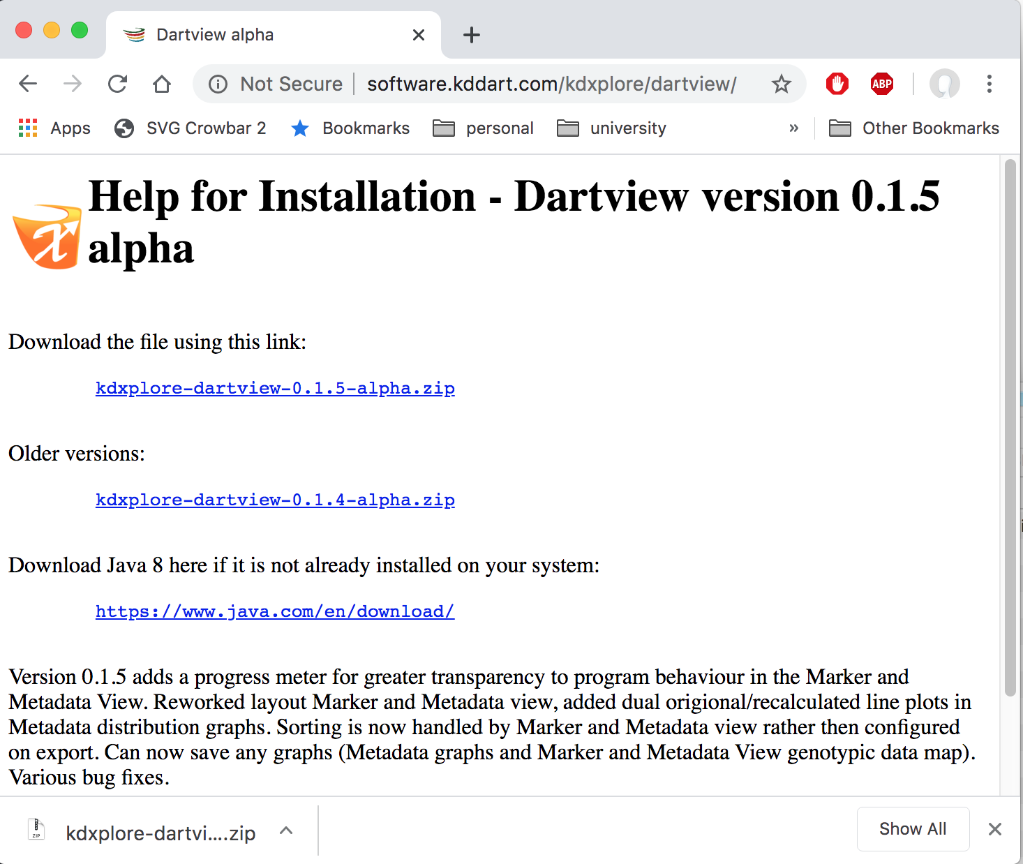
Prior to using the application, KDXplore requires Java to be installed on your computer. We recommend installing from https://www.java.com/en/download/.

If you have Java installed, you can download KDXplore-DArTView from http://software.kddart.com/kdxplore/dartview/.

Sample Fields Window (select to zoom)

The application is bundled as a ZIP archive which will need to be extracted after downloading:

Sample Fields Window (select to zoom)

To launch, open kdxplore.jar with Java:

Sample Fields Window (select to zoom)

This should load the KDXplore Main Window which houses all available KDX plugins. For this KDXplore version, we just have the DArTView plugin.

To launch DArTView from the KDXplore Main Window, just click the DArTView icon.

Launching DArTView from KDXplore

This should open DArTView, ready to import a new or recent marker data file:

Launching DArTView from KDXplore

Importing a Marker Data File

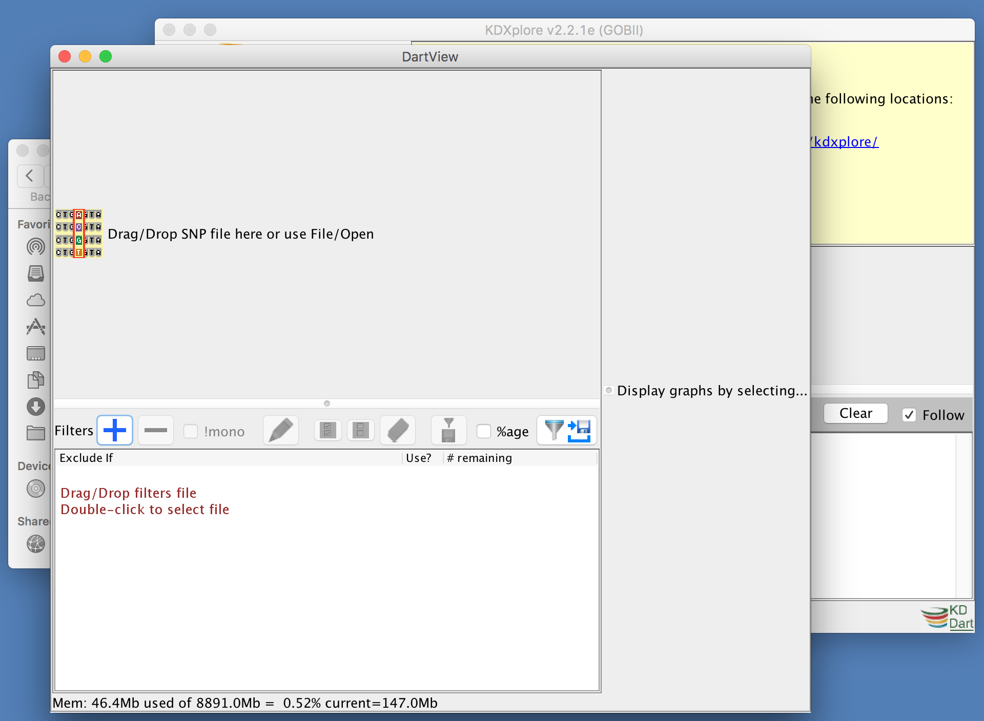
The first step to working with any data in DArTView is to import a marker data file. This section demonstrates how to import marker data files into DArTView.

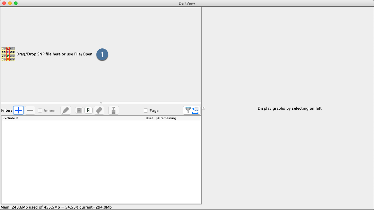
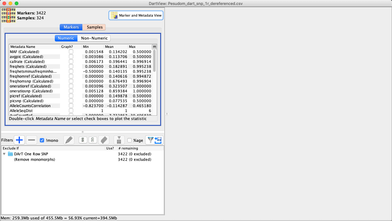
Empty DArTView (select to zoom)

Empty DArTView

To import a marker data file, you can either:

• Open DArTView and locate the marker data file that you would like to import. Click+drag the file to the File Panel in DArTView.

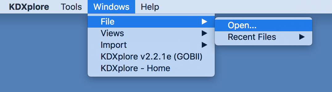
• Alternatively, open dartview via the application menu: * Windows->File->Open…

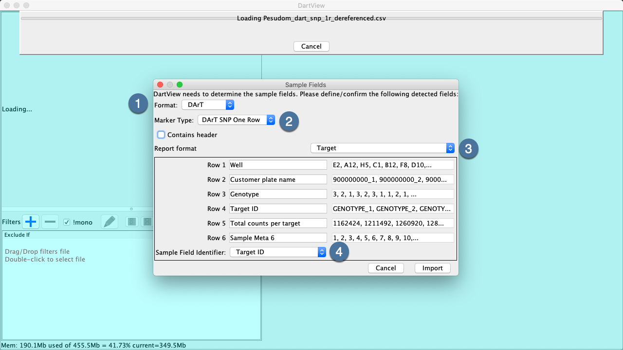
DArTView will attempt to automatically recognize your file and proceed to open it, but in case of ambiguity you’ll be prompt with the Import Marker Data Wizard. The wizard will require users to specify their marker data’s format, marker type, Report format (DArT only) and to identify sample metadata.

The next section details the steps of the Marker Data Import Wizard:

Sample Fields Window (select to zoom)

Note: Incorrect configuration can lead to incorrect metadata calculation

Imported Marker Data File (select to zoom)

DArTView Main Window

The DArTView Main Window displays an opened file, as well as filters and graphs that have been applied.

DArTView Main Window (select to zoom)

Panels of the DArTView Main Window

Item	UI Element	Description
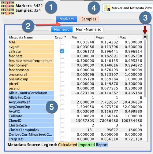
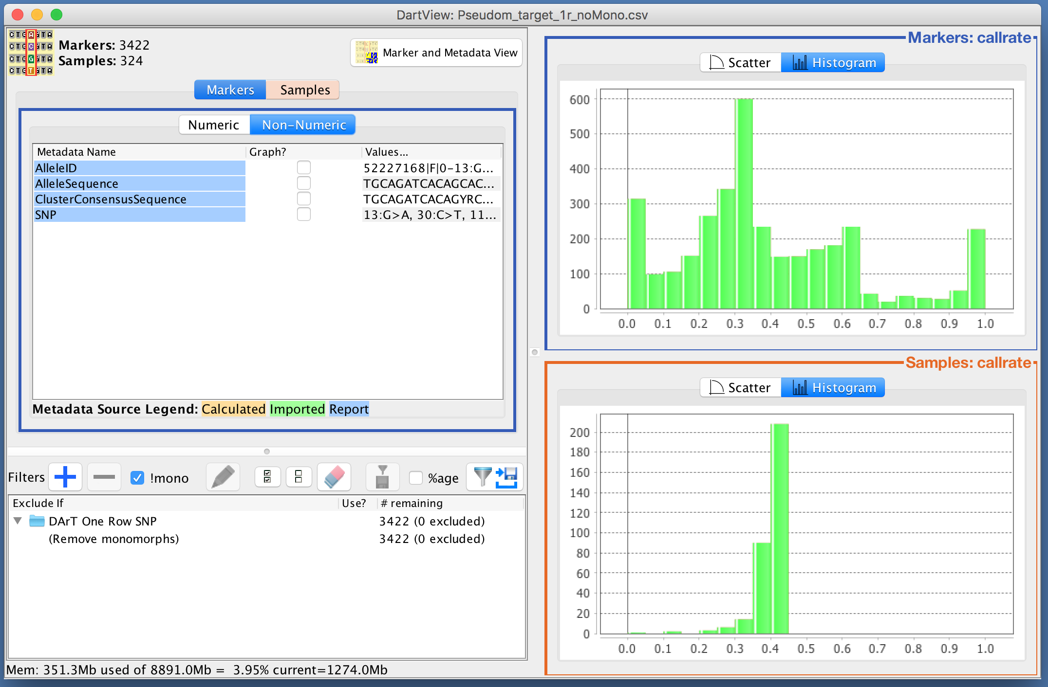
	Metadata Panel	Lists metadata that is organised into markers/samples with subsections numeric/non-numeric each. Checked metadata are displayed as a graphs in the Graphs Panel.
	Filters Panel	Lists all active/unactive filters that have been added to the file and provides options for managing these filters.
	Graphs Panel	Displays scatter and histograms plots based on the filters applied to a file.

Viewing Metadata Statistics

Data can be viewed after it is loaded from a marker data file. The options for viewing data are outlined in the image and table below:

Viewing Data (select to zoom)

Viewing Data

Item	UI Element	Description
	Report Counts	The total number of markers and samples are displayed here.
	Metadata Tabs	Select either the Markers Tab or the Samples Tab to view metadata on markers or samples from the report. The Numeric Tab and Non-Numeric Tab allows the user to view numeric and non-numeric metadata.
	Stats Button	The Metadata Panel in the above image displays only basic metadata stats. Select the Stats Button to choose the all stats option which displays all metadata stats available.
	Marker and Metadata View Button	This button will open a window called the Marker and Metadata View where data can be graphed. See the section below for more information.
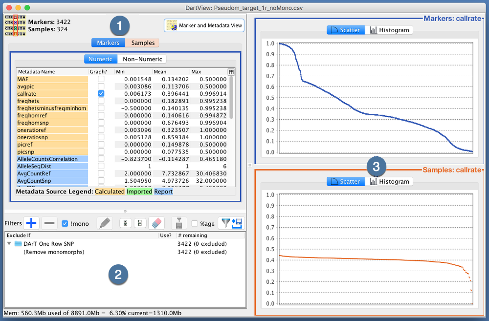
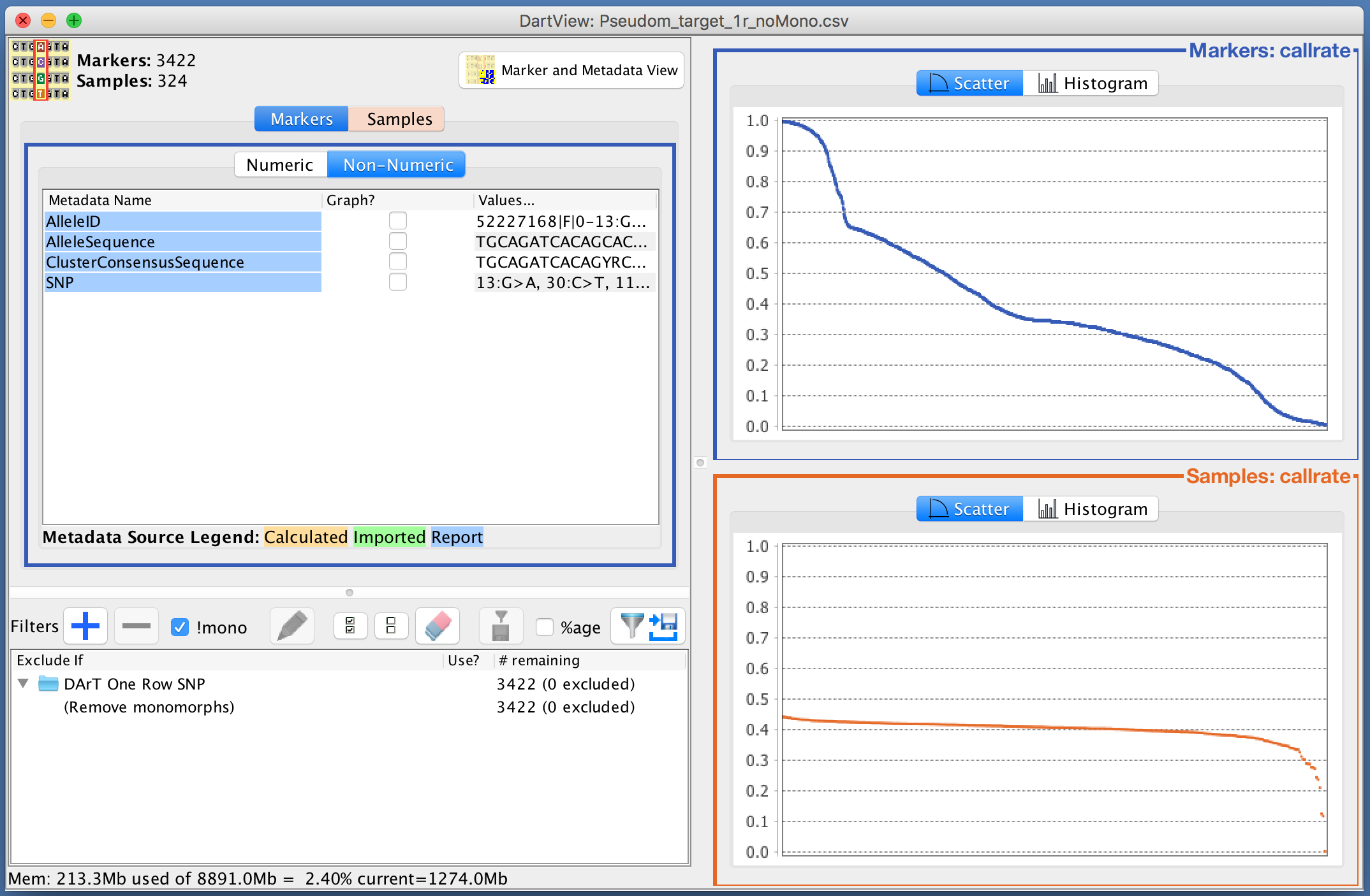
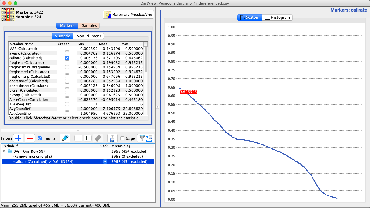
	Metadata Panel	This panel displays metadata according to what tabs the user has selected to view. Select the checkbox or double-click on any of the rows to display further information on the metadata. This is demonstrated in the image below where the callrate is selected and displayed.

Numeric Summary Statistics

Statistic	Description
Min	The minimum value for this metadata statistic
Mean	The mean value for this metadata statistic
Max	The maximum value for this metadata statistic
Extended: Q1	First interquartile range. The “middle” value in the first half of the rank-order data set
Extended: Median	Second interquartile range. The “middle” value of the rank-order data set
Extended: Q3	Third interquartile range. The “middle” value in the second half of the rank-order data set
Extended: Variance	The sample variance of the statistic: :raw-latex:`\frac{1}{N-1}\sum_i^N (\overline{X} - X_i)^2`
Extended: Std Dev	The sample standard deviation of the statistic: :raw-latex:`\sqrt{\frac{1}{N-1}\sum_i^N (\overline{X} - X_i)^2}`
Extended: Std Err	The sample standard deviation of the statistic: :raw-latex:`\frac{\sqrt{\frac{1}{N-1}\sum_i^N (\overline{X} - X_i)^2}}{\sqrt{N}}`

Non-numeric Summary Statistics :widths: 1 70 :header-rows: 1

Statistic	Description
Values	Displays some entries of the metadata

Metadata Source Types

Source	Description
Calculated	Metadata has been calculated using DArTView’s internal set of calculators for this data format
Report	Metadata was imported from report
Imported	Metadata was imported via “Import Metadata Wizard”

Viewing Graphed Metadata

Each metadata row can be viewed in more detail in different graphs located in the Graphs Panel. Select the checkbox or double-click on any of the rows to display more information in the form of scatter plots and histograms of the data.

The images below are examples of the callrate being graphed as both a scatter plot and a histogram. The data is displayed in descending order as that is what order it was designated in the Metadata Panel. There are also checkboxes along the bottom on the scatter plot which provide options for marking summary statistics of the data. The median is marked in this example and can be seen with the blue line through the scatter plot.

Scatter Plot (select to zoom)

Histogram (select to zoom)

Adding Filters

Filters can be used to refine the data set that is viewed in DArTView and can be saved for reuse. Filters can be either created or loaded from a previously saved filter file.

Filter Panel

The Filter Panel displays all active and unactive (Checked/Unchecked) filters and provides options for managing those filters. The filter panel will switch with the Markers or Samples tab. The image and table below outline the options that are available:

Filters Panel (select to zoom)

Filters Panel Options

UI Element	Description
Add New Filter Button	Displays the Add New Filter Window which provides options for creating a new filter.
Remove Filter Button	Removes the selected filter.
Remove Mono Checkbox (Markers only)	This is a special filter which is applied only after standard filters (Both markers and samples) are applied. A monomorphic marker is defined as a marker with only one allele visible across the samples (Ignore missing values). Such markers are considered uninformative and are often redundant in downstream analysis. The Remove Monomorphs Filter is always available by default and can’t be removed. However, this checkbox allows the user to enable/disable this filter.
Edit Filter Button	Opens the Edit Filter Window for editing a selected filter.
Check All Button	Enables all filters in the Filters Panel.
Uncheck All Button	Disables all filters in the Filters Panel.
Uncheck Not Applicable Filters Button	Disables all filters that are not applicable to the marker data file that is currently open.
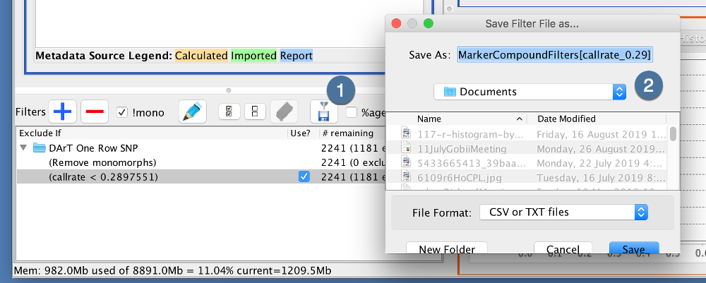
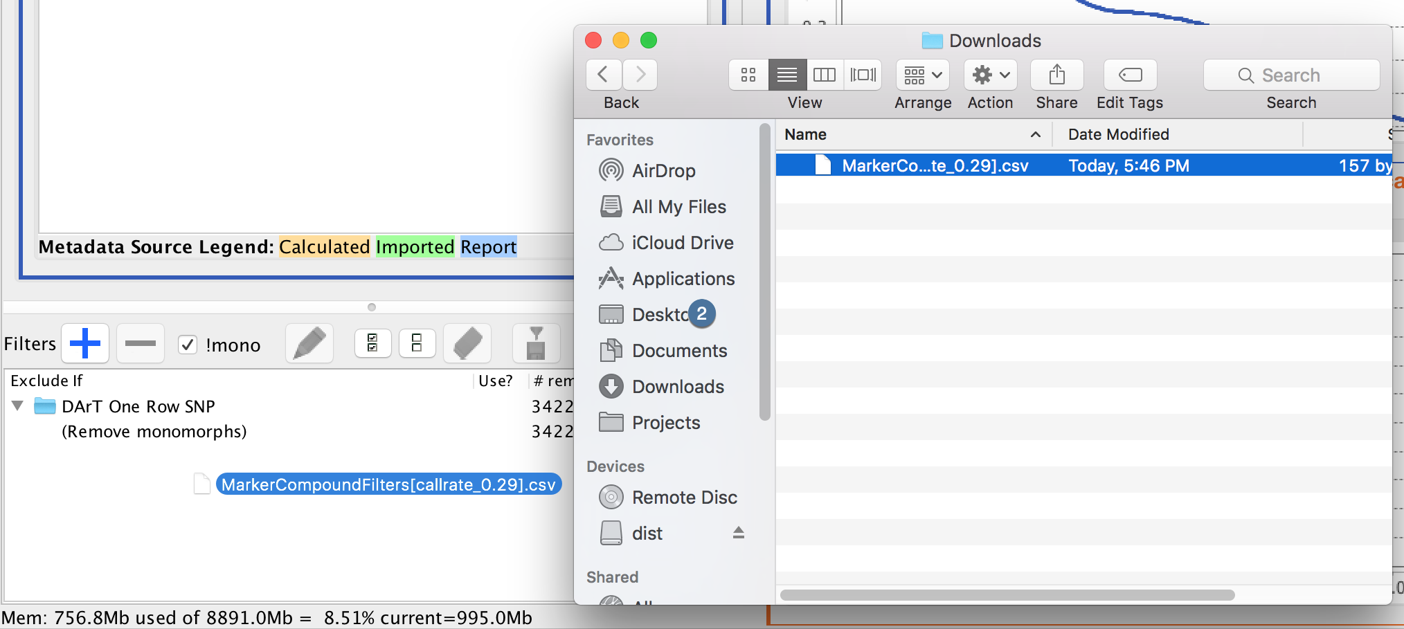
Export Filters Button	Provides options for exporting selected filters to a separate file so that they can be reused again.
Percentage Checkbox	By default, each filter will display the number of data points that are excluded if the filter is active. This checkbox will display the number as a percentage rather than a count.
Export Data with Filters Button	Provides options for exporting data with the filters that have been applied.

Exporting and Importing Filters

Exporting

Saving a filter will create a file with saved filters from the current session. This can used for future use.

Creating a Filter in the Filter Panel (select to zoom)

Exporting to a Filter File

1.	After creating your filters, click the Export Filters Button
2.	Select a location to save your filter file

Importing

Importing a filter file is performed by dragging the filter file from file explorer and dropping into the Filter panel

Importing a Filter file

Creating New Filters

There are two approaches to creating new filters. The first is via the Filter panel and the secondary via the graph.

Creating a Filter in the Filter Panel

Filters can be created in the Filters Panel without needing to view any graphed data. See the instructions below for more information:

Creating a Filter in the Filter Panel (select to zoom)

Creating a Filter in the Filters Panel 1/2

Step	Action
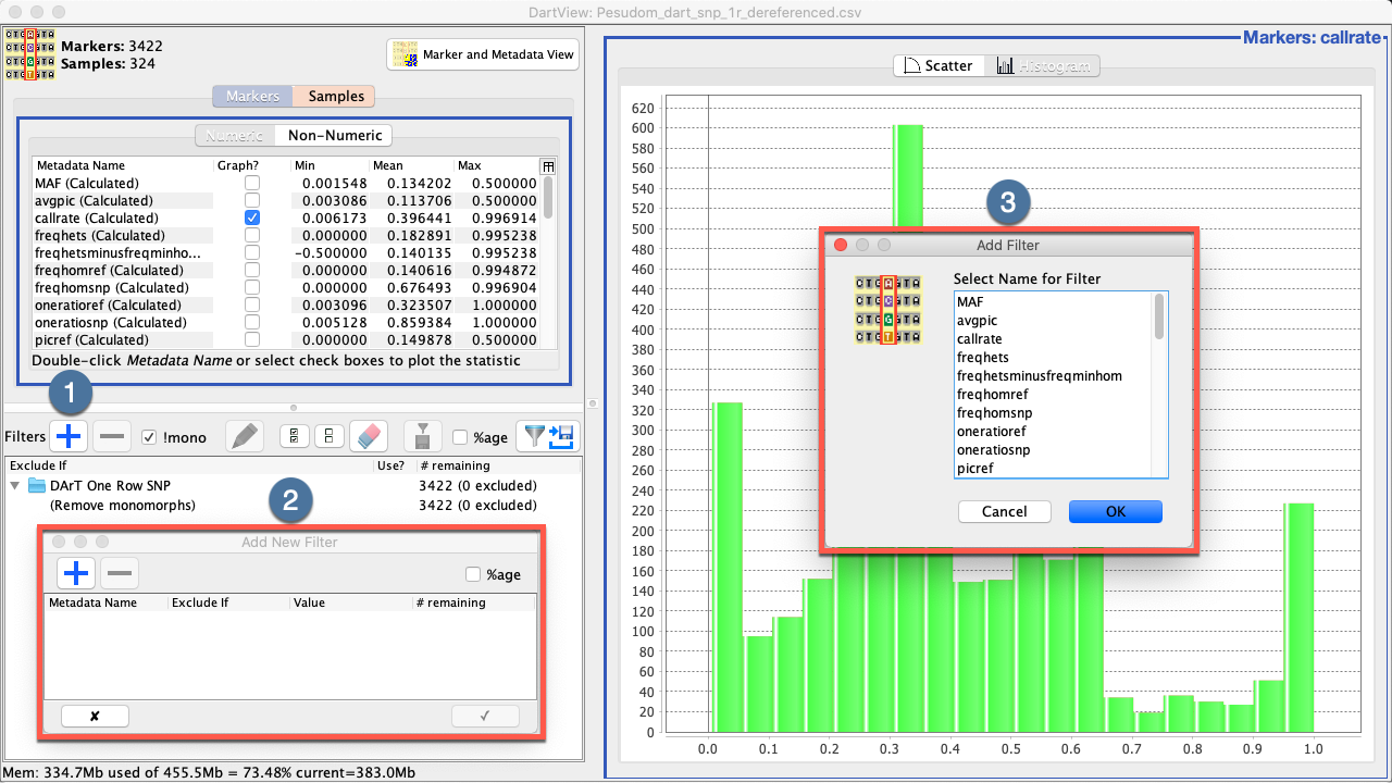
1.	Select the Add Filter Button in the Filter Panel at to begin creating a new filter. This will open the Add New Filter Window at .
2.	Select the Add Filter Button within the Add New Filter Window to start creating a filter condition. Each filter can have one or more conditions. It will open the Add Filter Window at .
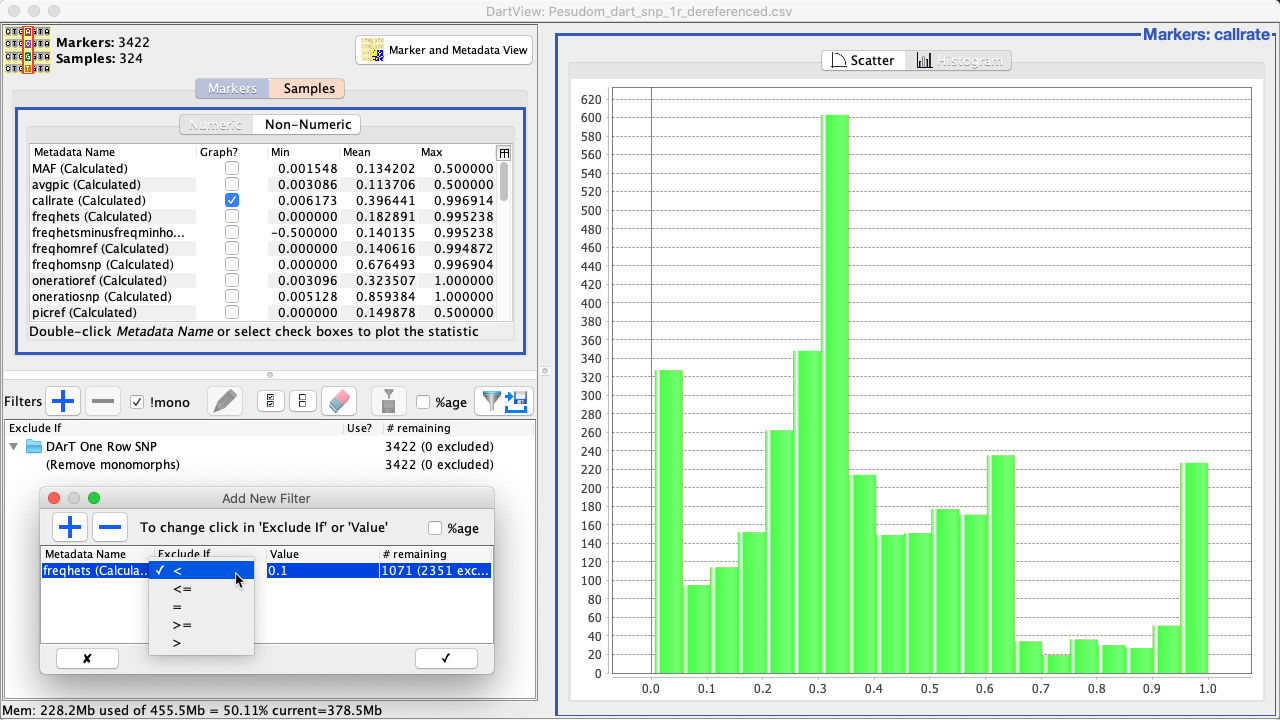
3.	Choose the metadata for the filter then select the Ok Button to finalise the selection. The Add New Filter Window will be updated as seem in the image below.

Creating a Filter Condition (select to zoom)

Creating a Filter in the Filters Panel 2/2

4.	The filter condition can be edited by double-clicking the Metadata Name, Exclude If (such as in the above image), and Value fields.
5.	Select the Confirm Button (the tick) to finalise the creation of the filter. The graph will be updated such as in the image below.

Filtered Data (select to zoom)

Tip

Both the scatter plot and histogram will be affected by applied filters.

Creating a Filter in a Histogram or Scatter Plot

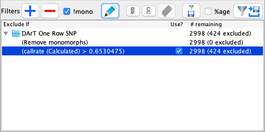
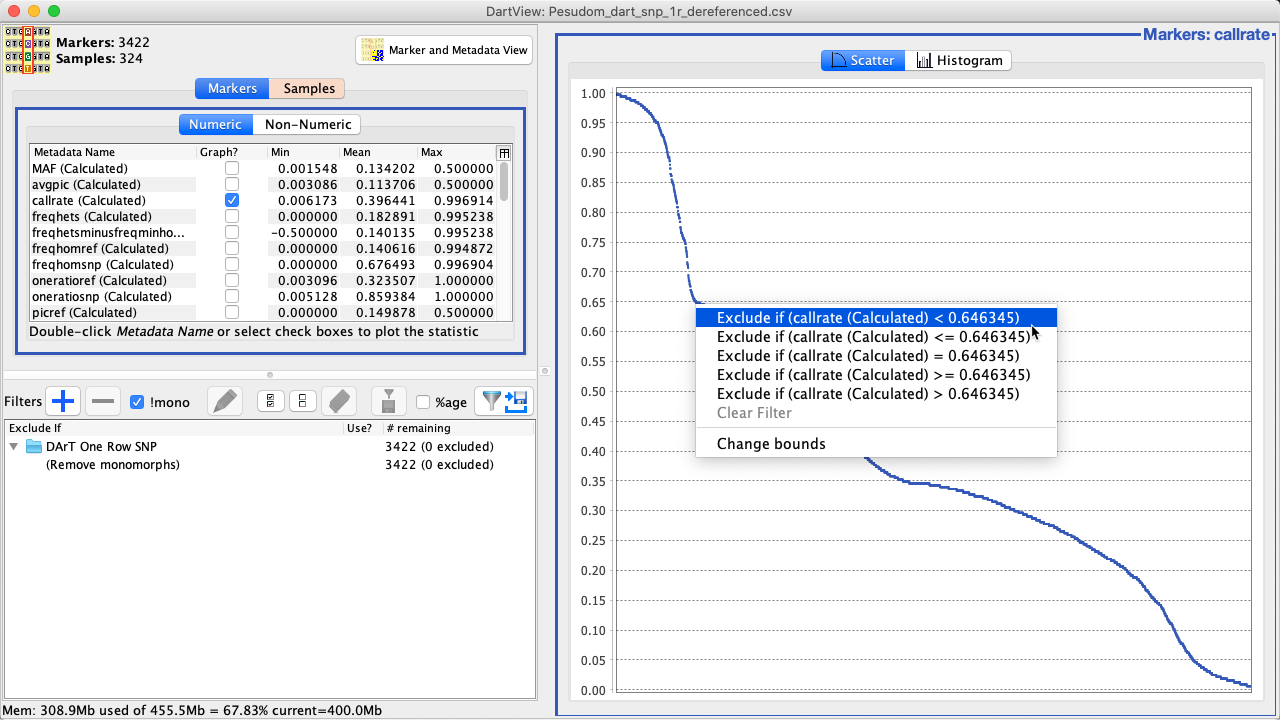
New filters can also be created within a histogram or scatter plot. This allows users to filter based on the graph they are viewing. See the instructions below for more information:

Filtering Data from a Graph (select to zoom)

Creating a Filter in a Histogram or Scatter Plot

Step	Action
1.	Open a histogram or scatterplot from the Metadata Panel by selecting the relevant checkbox.
2.	Right+click in a section within the graph that you want to place a filter (such as in the above image). Filtering (and other) options will be presented.
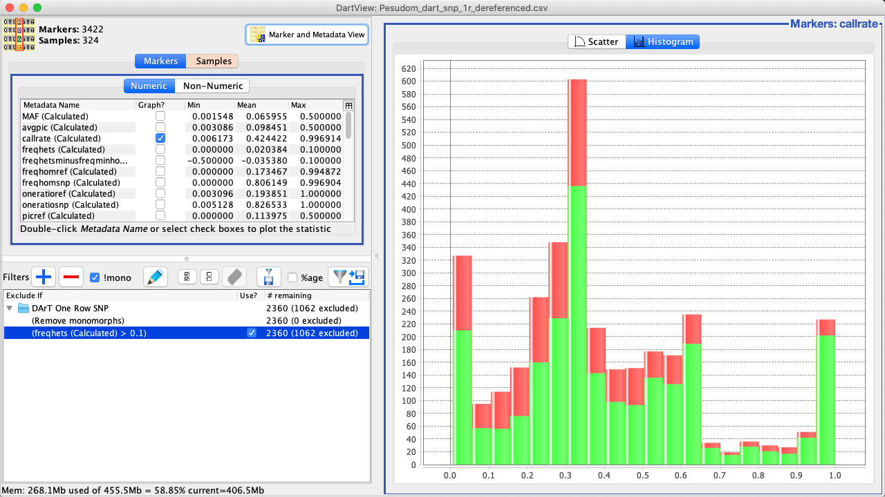
3.	Select a filtering option. This will add and apply the filter immediately as seen in the image below.

Filtered Data (select to zoom)

Importing Additional Data Files

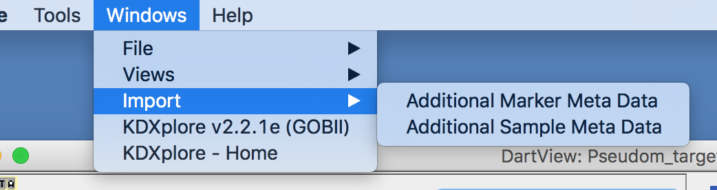
It is also possible to import additional marker or sample metadata files which are appended to an existing, open marker data file. See the instructions below for how to import additional data:

Additional metadata can be imported in the form of a CSV table data. This can be with or without a header.

To begin, choose to import either Marker metadata or Sample metadata via the menu:

Sample Fields Window 1/2 (select to zoom)

Sample Fields Window 1/2 (select to zoom)

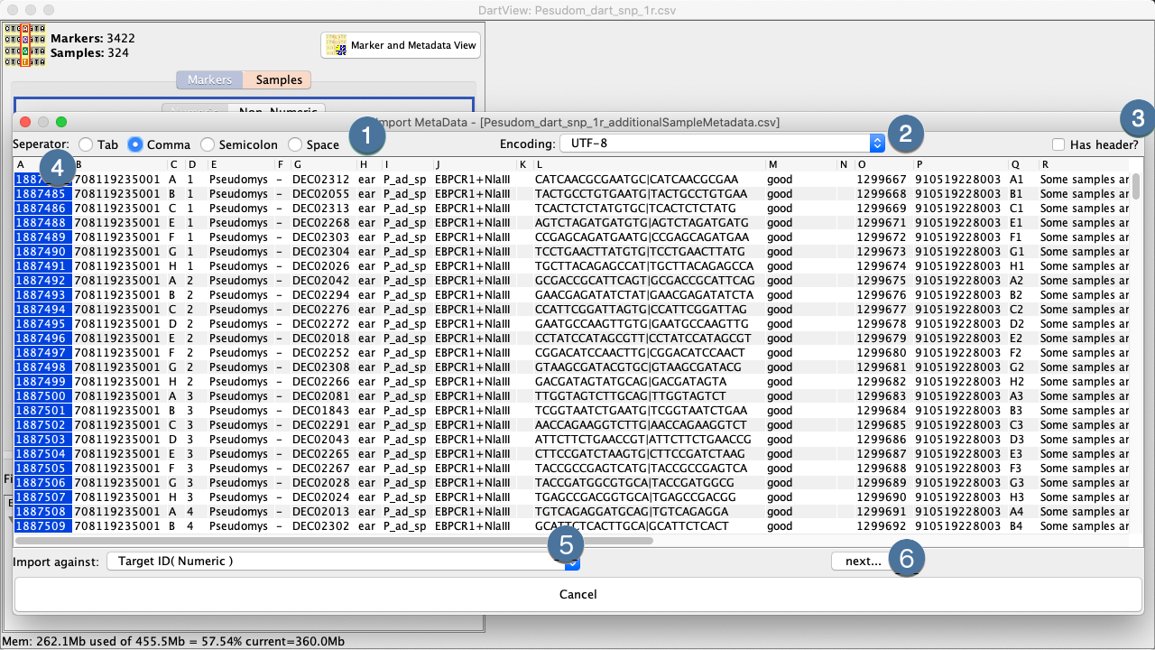
This will prompt you to specify the CSV to import.

Adding Marker Data Files to DArTView 2/2

1.	Select the delimiter of your CSV
2.	Specify the encoding. Typically, CSVs are UTF-8
3.	Specify whether the file contains a header or or not. Headerless columns with be identified by column ID.
4.	Click the header of the field that will be used to align against an existing metadata field. This field must have unique values to ensure the imported metadata can be mapped (Note: Your metadata file does not need to be in the same order as your Marker Data File).
5.	Select which exiting metadata field in DArTView to align your new data against. Similarly, this field must have unique values
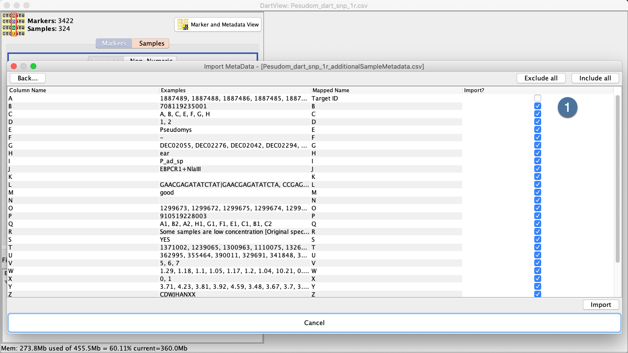
6.	Select the Import Button to finalise the import of the file which will take you to the DArTView Main Window which should now look something like:

Sample Fields Window 2/2 (select to zoom)

The Marker and Metadata View

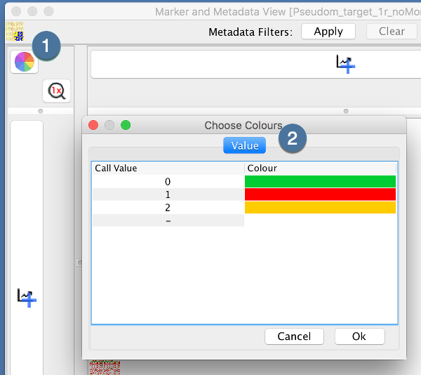
The Marker and Metadata View provides a full coloured visualisation of the genotypic data. Each genotype data point has a representative color. Colouring is configured by the “Choose Colours” dialog:

Marker and Metadata View (select to zoom)

Selecting colors

Step	Action
1.	Open the “Choose Colours” Dialog by clicking the color wheel
2.	Set each color of each “Call Value” by clicking the “Colour”

Clicking “Ok” will update the genotype data points displayed.

The Genotypic Data Map

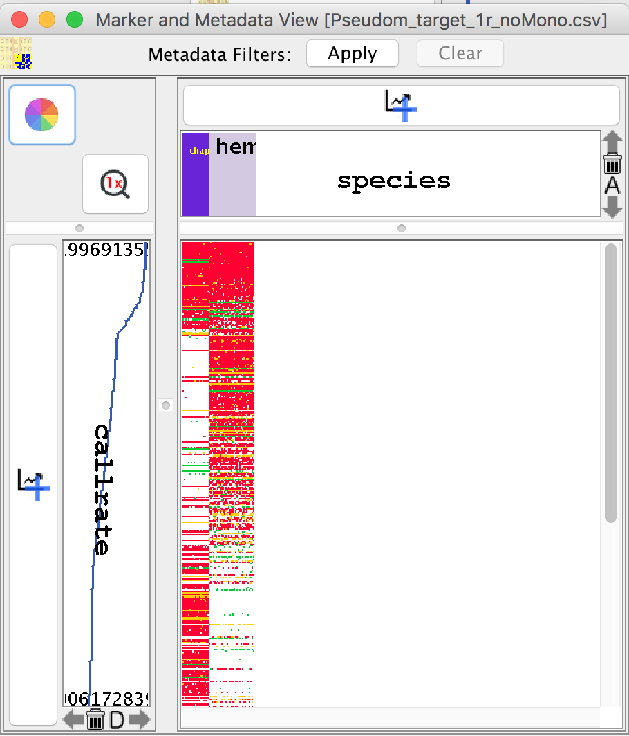
The Genotypic Data Map provides a contrasting image of the marker data before and after filtering. Along with sorting capabilities, this feature provides a quick perspective of the dataset.

In the image below, the Genotypic Data Map is sorted by marker call rate and a species sample metadata which had been imported via the “Import Additional Metadata Wizard”.

Marker and Metadata View (select to zoom)

Graphing Data in the Marker and Metadata View

Metadata distributions of either Markers or Samples can be added alongside the Genotypic Data Map.

See the below table for information on how to graph data in the Marker and Metadata View.

Graphing Data in the Marker and Metadata View (select to zoom)

Graphing Data in the Marker and Metadata View

Step	Action
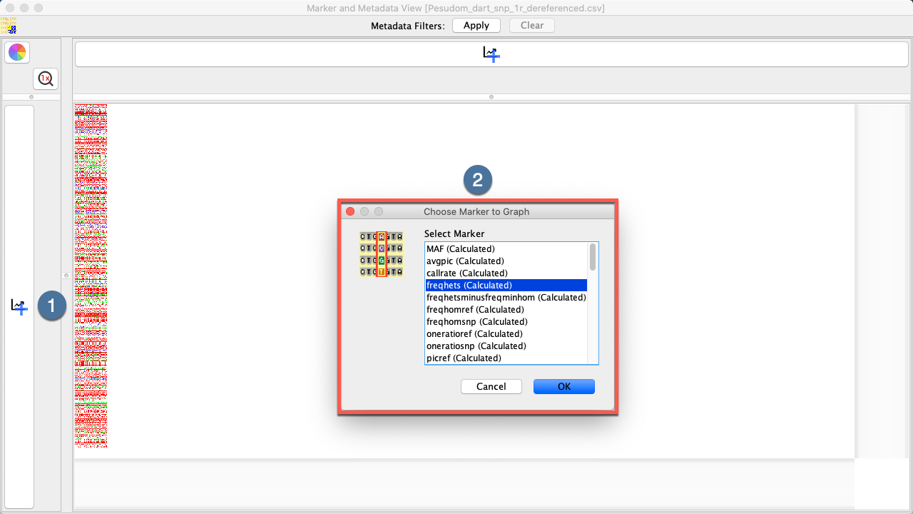
1.	Open the Marker and Metadata View Window to view genotypic data.
2.	Select the Add Graph Button for markers (on the left like in the example) or samples (on the top) which will display graphing options seen at .
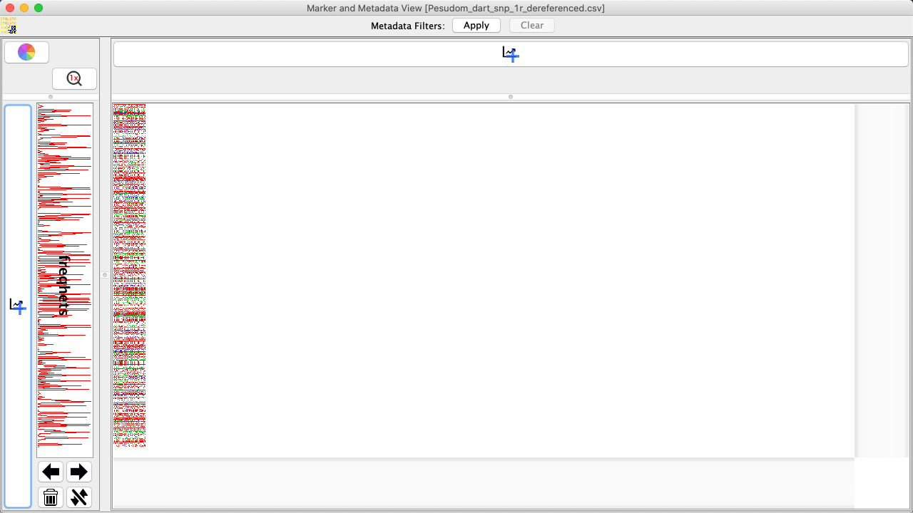
3.	Select a graph option and then the OK Button. The new graph will be created and applied to the appropriate location. The below image shows that the example graph looks like.

Graph Added to Marker and Metadata View(select to zoom)

Graph and Viewing Options

There are display options available once a graph has been added. The following options are available:

Graph Options of the Marker and Metadata View

UI Element	Description
/ Increase Priority	As multiple graphs can be applied to the data, this option increases the priority of the selected graph.
/ Decrease Priority	Descreases the priority of the selected graph.
Delete Graph	Deletes the selected graph.
Sort	Cycles through the following sorting options for the selected graph: Unsorted; Ascending; and Descending.
Change Colours	Displays a window with options for changing the colour for each call value.
Reset Zoom	Sets the zoom level to 1x (normal). There are more zoom options in the following section.

Genotype Data Points

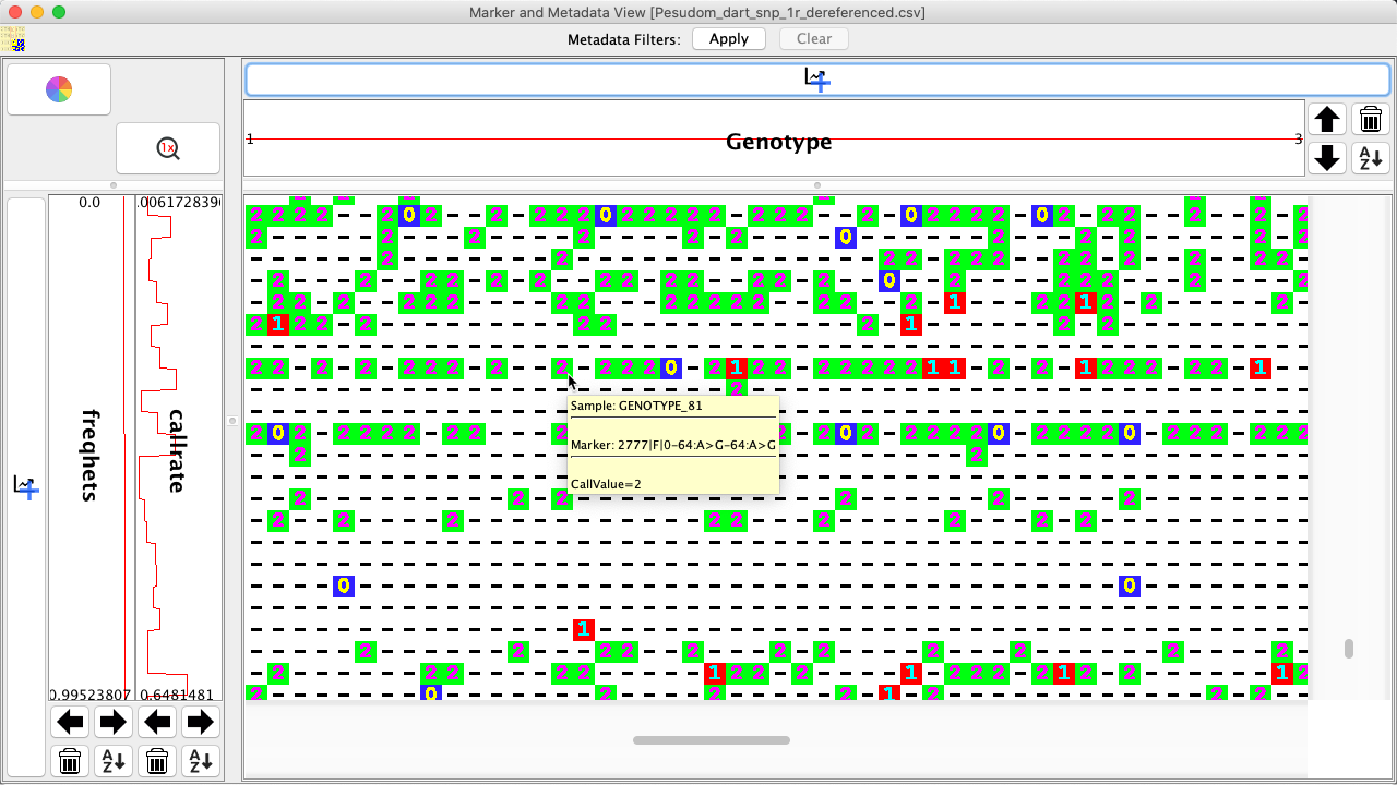
Samples, markers, and call values can be easily viewed in the Marker and Metadata View. Hold the mouse over a genotype data point (this may be easier if zoomed in) to display the sample, marker, and call value as seen in the image below:

Genotype Data Point Information View(select to zoom)

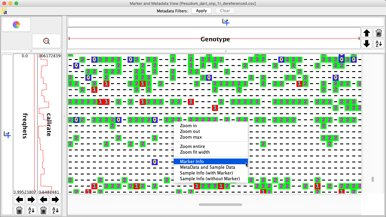
Right+clicking on a genotype data point will also provide options which are shown in the image below and listed in the the table below that:

Genotype Data Point Options(select to zoom)

Call Value Options

Option	Description
Zoom In	Zoom in closer to selected call value.
Zoom Out	Zoom out from selected call value.
Zoom Max	Maximised the zoom depth (Which will display values as text) onto the focused location
Zoom Entire	Fits the entire genotypic matrix into view
Zoom Fit Width	Fits the width of the genotypic matrix into the window Metadata and Sample Data: Shows marker and sample metadata. Need to make it clear which is marker and which is sample
Save as PNG…	Saves the current Genotypic Data Map with adjacent metadata distributions as a PNG
Show metadata for genotypic data point	All information for the selected marker which includes anything that was imported to DArTView.

Exporting Marker Data

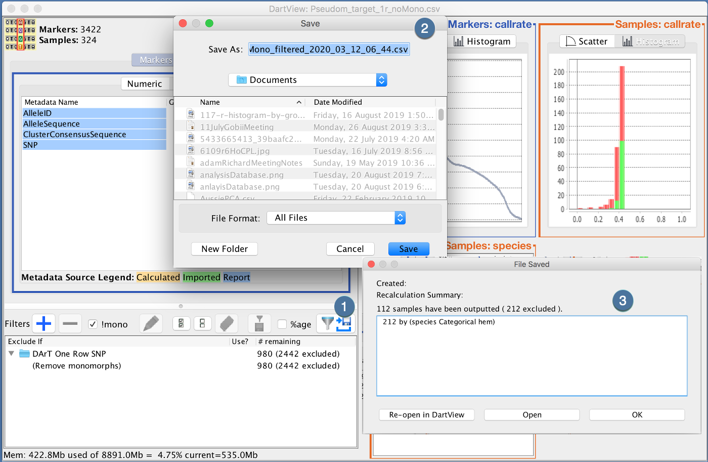
At any point, you can export your filtered marker data. The Export feature will subset your Marker Data file based on your filters and sorted in the order represented in the Marker and Metadata View.

Genotype Data Point Options(select to zoom)

Exporting a Marker Data File

Step	Description
1	Click the “Export data applying selected Filters”
2	Select a location to save
3	Once DArTView has completed exporting your filtered file, you can choose to re-import back in DArTView, open using your default application or continue with the currently loaded marker data file